设计教育培训seo基础培训
—— 分而治之,逐个击破
把特征空间划分区域
每个区域拟合简单模型
分级分类决策
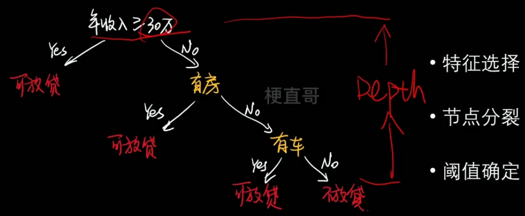
1、核心思想和原理

- 举例:
- 特征选择、节点分类、阈值确定
2、信息嫡
熵本身代表不确定性,是不确定性的一种度量。
熵越大,不确定性越高,信息量越高。
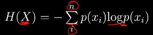
为什么用log?—— 两种解释,可能性的增长呈指数型;log可以将乘法变为加减法。
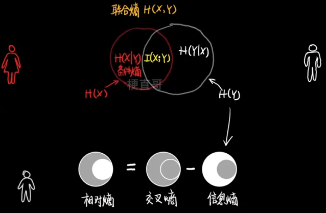
联合熵 的物理意义:观察一个多变量系统获得的信息量。
条件熵 的物理意义:知道其中一个变量的信息后,另一个变量的信息量。
给定了训练样本 X ,分类标签中包含的信息量是什么。

信息增益(互信息)
代表了一个特征能够为一个系统带来多少信息。

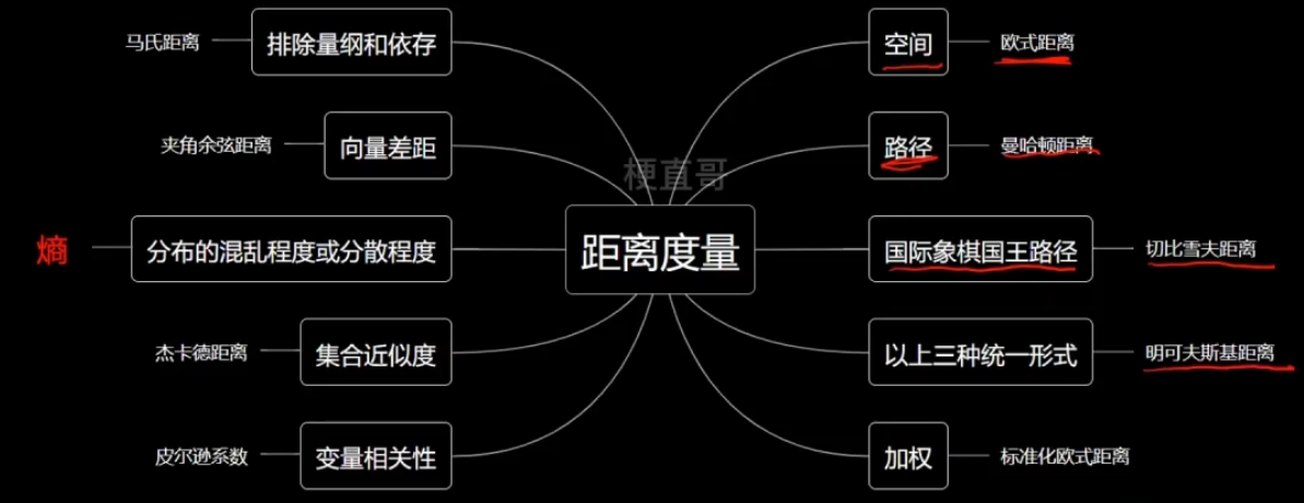
熵的分类

熵的本质:特殊的衡量分布的混乱程度与分散程度的距离
二分类信息熵:
二分类信息熵
import numpy as np
import matplotlib.pyplot as plt
def entropy(p):return -(p * np.log2(p) + (1 - p) * np.log2(1 - p))plot_x = np.linspace(0.001, 0.999, 100)
plt.plot(plot_x, entropy(plot_x))
plt.show() 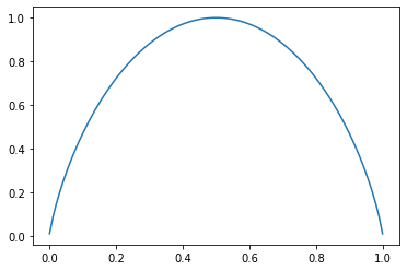
决策树的本质

3、决策树分类代码实现
数据集
from sklearn.datasets import load_irisiris = load_iris()
x = iris.data[:, 1:3]
y = iris.target
plt.scatter(x[:,0], x[:,1], c = y)
plt.show()
3.1、sklearn中的决策树
from sklearn.tree import DecisionTreeClassifierclf = DecisionTreeClassifier(max_depth=2, criterion='entropy')
clf.fit(x, y)DecisionTreeClassifier
DecisionTreeClassifier(criterion='entropy', max_depth=2)
决策边界绘制的代码:
def decision_boundary_plot(X, y, clf):axis_x1_min, axis_x1_max = X[:,0].min() - 1, X[:,0].max() + 1axis_x2_min, axis_x2_max = X[:,1].min() - 1, X[:,1].max() + 1x1, x2 = np.meshgrid( np.arange(axis_x1_min,axis_x1_max, 0.01) , np.arange(axis_x2_min,axis_x2_max, 0.01))z = clf.predict(np.c_[x1.ravel(),x2.ravel()])z = z.reshape(x1.shape)from matplotlib.colors import ListedColormapcustom_cmap = ListedColormap(['#F5B9EF','#BBFFBB','#F9F9CB'])plt.contourf(x1, x2, z, cmap=custom_cmap)plt.scatter(X[:,0], X[:,1], c=y)plt.show()decision_boundary_plot(x, y, clf)
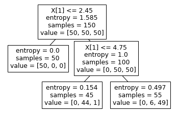
from sklearn.tree import plot_tree
plot_tree(clf)
[Text(0.4, 0.8333333333333334, 'X[1] <= 2.45\nentropy = 1.585\nsamples = 150\nvalue = [50, 50, 50]'),Text(0.2, 0.5, 'entropy = 0.0\nsamples = 50\nvalue = [50, 0, 0]'),Text(0.6, 0.5, 'X[1] <= 4.75\nentropy = 1.0\nsamples = 100\nvalue = [0, 50, 50]'),Text(0.4, 0.16666666666666666, 'entropy = 0.154\nsamples = 45\nvalue = [0, 44, 1]'),Text(0.8, 0.16666666666666666, 'entropy = 0.497\nsamples = 55\nvalue = [0, 6, 49]')]
3.2、最优划分条件
from collections import Counter
Counter(y)
Counter({0: 50, 1: 50, 2: 50})
def calc_entropy(y):counter = Counter(y)sum_ent = 0for i in counter:p = counter[i] / len(y)sum_ent += (-p * np.log2(p))return sum_entcalc_entropy(y)1.584962500721156
def split_dataset(x, y, dim, value):index_left = (x[:, dim] <= value)index_right = (x[:, dim] > value)return x[index_left], y[index_left], x[index_right], y[index_right]def find_best_split(x, y):best_dim = -1best_value = -1best_entropy = np.infbest_entropy_left, best_entropy_right = -1, -1for dim in range(x.shape[1]):sorted_index = np.argsort(x[:, dim])for i in range(x.shape[0] - 1): # x列数value_left, value_right = x[sorted_index[i], dim], x[sorted_index[i + 1], dim]if value_left != value_right:value = (value_left + value_right) / 2x_left, y_left, x_right, y_right = split_dataset(x, y, dim, value)entropy_left, entropy_right = calc_entropy(y_left), calc_entropy(y_right)entropy = (len(x_left) * entropy_left + len(x_right) * entropy_right) / x.shape[0]if entropy < best_entropy:best_dim = dimbest_value = valuebest_entropy = entropybest_entropy_left, best_entropy_right = entropy_left, entropy_rightreturn best_dim, best_value, best_entropy, best_entropy_left, best_entropy_rightfind_best_split(x, y)(1, 2.45, 0.6666666666666666, 0.0, 1.0)
x_left, y_left, x_right, y_right = split_dataset(x, y, 1, 2.45)find_best_split(x_right, y_right)(1, 4.75, 0.34262624992678425, 0.15374218032876188, 0.4971677614160753)
4、基尼系数

基尼系数运算稍快;
物理意义略有不同,信息熵表示的是随机变量的不确定度;
基尼系数表示在样本集合中一个随机选中的样本被分错的概率,也就是纯度。
基尼系数越小,纯度越高。
模型效果上差异不大。
二分类信息熵和基尼系数代码实现:
import numpy as np
import matplotlib.pyplot as plt
def entropy(p):return -(p * np.log2(p) + (1 - p) * np.log2(1 - p))def gini(p):return 1 - p ** 2 - (1 - p) ** 2plot_x = np.linspace(0.001, 0.999, 100)
plt.plot(plot_x, entropy(plot_x), color = 'blue')
plt.plot(plot_x, gini(plot_x), color = 'red')
plt.show()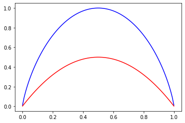
5、决策树剪枝
Chapter-07/7-6 决策树剪枝.ipynb · 梗直哥/Machine-Learning - Gitee.com
为什么要剪枝?
复杂度过高。
预测复杂度:O(logm)
训练复杂度:O(n x m x logm)
logm为数的深度,n为数据的维度。
容易过拟合
为非参数学习方法。
目标:
降低复杂度
解决过拟合
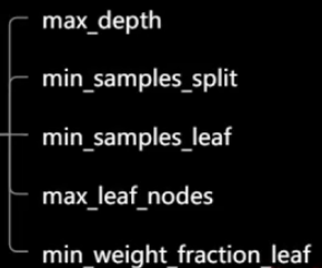
手段:
限制深度(结点层数)
限制广度(叶子结点个数)
—— 设置超参数
6、决策树回归
基于一种思想:相似输入必会产生相似输出。
取节点平均值。

6.1、决策树回归代码实现
import matplotlib.pyplot as plt
import numpy as np
from sklearn import datasets
from sklearn.model_selection import train_test_split
import warnings
warnings.filterwarnings('ignore')boston = datasets.load_boston()
x = boston.data
y = boston.target
x_train, x_test, y_train, y_test = train_test_split(x, y, random_state=233)from sklearn.tree import DecisionTreeRegressorreg = DecisionTreeRegressor()
reg.fit(x_train,y_train)DecisionTreeRegressor
DecisionTreeRegressor()
reg.score(x_test,y_test)0.7410680140563546
reg.score(x_train,y_train)1.0
6.2、绘制学习曲线
from sklearn.metrics import r2_scoreplt.rcParams["figure.figsize"] = (12, 8)
max_depth = [2, 5, 10, 20]for i, depth in enumerate(max_depth):reg = DecisionTreeRegressor(max_depth=depth)train_error, test_error = [], []for k in range(len(x_train)):reg.fit(x_train[:k+1], y_train[:k+1])y_train_pred = reg.predict(x_train[:k + 1])train_error.append(r2_score(y_train[:k + 1], y_train_pred))y_test_pred = reg.predict(x_test)test_error.append(r2_score(y_test, y_test_pred))plt.subplot(2, 2, i + 1)plt.ylim(0, 1.1)plt.title("Depth: {0}".format(depth))plt.plot([k + 1 for k in range(len(x_train))], train_error, color = "red", label = 'train')plt.plot([k + 1 for k in range(len(x_train))], test_error, color = "blue", label = 'test')plt.legend()plt.show()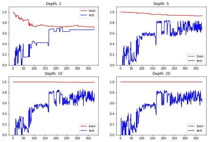
6.3、网格搜索
from sklearn.model_selection import GridSearchCVparams = {'max_depth': [n for n in range(2, 15)],'min_samples_leaf': [sn for sn in range(3, 20)],
}grid = GridSearchCV(estimator = DecisionTreeRegressor(), param_grid = params, n_jobs = -1
)grid.fit(x_train,y_train)GridSearchCV
GridSearchCV(estimator=DecisionTreeRegressor(), n_jobs=-1,param_grid={'max_depth': [2, 3, 4, 5, 6, 7, 8, 9, 10, 11, 12, 13,14],'min_samples_leaf': [3, 4, 5, 6, 7, 8, 9, 10, 11, 12,13, 14, 15, 16, 17, 18, 19]})
estimator: DecisionTreeRegressor
DecisionTreeRegressor()
DecisionTreeRegressor
DecisionTreeRegressor()
grid.best_params_{'max_depth': 5, 'min_samples_leaf': 3}
grid.best_score_0.7327442904059717
reg = grid.best_estimator_reg.score(x_test, y_test)0.781690085676063
7、优缺点和适用条件
优点:
符合人类直观思维
可解释性强
能够处理数值型数据和分类型数据
能够处理多输出问题
缺点:
容易产生过拟合
决策边界只能是水平或竖直方向

不稳定,数据的微小变化可能生成完全不同的树
参考于
Chapter-07/7-4 决策树分类.ipynb · 梗直哥/Machine-Learning - Gitee.com